Portfolio Management: Fee Generation in AMMs

In the previous article, we examined the concept of Portfolio Value Functions (PVFs) in the context of Constant Function Market Makers (CFMMs), and how Liquidity Pool Tokens (LPTs) (also called liquidity provider shares) can be viewed as automatically managed portfolios. By understanding the relationship between CFMM trading functions and PVFs, as outlined in the Replicating Market Makers paper, we gained insights into how Liquidity Providers (LPs) can better anticipate the potential risks and rewards associated with their provision to a CFMM. Additionally by treating the LPT as a tradeable asset, we enabled the creation of more complex portfolio strategies including convex portfolios. This concept was further explored in the context of our previous CFMM implementation, RMM-CC, in Replicating Portfolios: Constructing Permissionless Derivatives.

In this blog post, we will build on that foundation and explore the more nuanced aspect of liquidity provision in a CFMM: how fees are generated on the CFMM and how does your liquidity distribution affect that? Our aim here is to provide an accessible yet comprehensive explanation of fee growth in a CFMM and how path dependence plays a crucial role within the process. Examining fee growth is crucial to undertanding the payoff of liquidity provision. While avoiding a heavy focus on the underlying mathematics, we will dive into the fundamental concepts and factors that define fee growth in CFMMs, including path dependency and its impact on the efficiency of liquidity provision in a CFMM.

Fee Growth in CFMMs

In a CFMM, the swap fee is a crucial element that encourages users to provide liquidity to the protocol. Although it's possible for a CFMM to operate without a swap fee, most live implementations incorporate one, typically ranging from 0.01% to 0.30% of the swap volume. This fee serves as an extra incentive for users to contribute liquidity to the pool.

To better understand how the swap fee is generated, imagine a swap taking place within a CFMM. When a user initiates a swap, they pay a small percentage of the swap amount as a fee, based on the fee rate set by the protocol. This fee is then deducted from the user's input amount, and the trade is executed with the remaining value.

Instead of being paid directly to the LPs, the swap fees can be reinvested back into the liquidity pool. By doing so, the protocol effectively increases the total value of assets in the pool, which benefits liquidity providers in the long run.

It's important to note that the swap fees are directly related to the changes in price, rather than the price itself. This is due to the fact that the pool price and reserves in CFMMs maintain a one-to-one relationship. As a result, any time a trade occurs and reserves change, the price also changes. This differs from the constant sum market maker, which has a single fixed price.

Because fees are tied directly to price changes rather than price itself, it becomes hard to predict the ultimate fee growth a CFMM position will have without also knowing the ultimate path price takes on the CFMM. This property is known as path dependence, which implies that the start and end prices aren't enough information to determine how much fees were generated. Understanding path dependence is crucial for LPs, as it affects their potential earnings and highlights the importance of considering factors beyond just the final price of the assets when making allocation decisions.

Path Dependence

Path dependence, in the context of CFMMs, refers to the phenomenon where the fees generated and the value of an LPT depend not only on the starting and ending prices but also on all the intermediate prices that the pool hits between these points. In a CFMM without a swap fee, however, the portfolio value depends only on the final price of the pool. This indicates the path dependence arises from the relationship between the trading function and the swap fee, and isn't a property of a CFMM itself. Let's illustrate how this property works through an example.

Illustration

Given that fees are tied directly to price changes, different price paths can lead to different fee outcomes for LPs. For instance, consider two scenarios with the same CFMM, same liquidity, and same start and end prices but different price paths:

1. In the first scenario, the price moves directly from the start price to the end price with no additional volatility. Our price path is $P_{\text{start}}\to P_{\text{end}}$
2. In the second scenario, the price experiences an additional fluctuation on the way from the start to end prices. Our price path is $P_{\text{start}}\to P_1\to P_{\text{start}}\to P_{\text{end}}$

Note that the price path in the first scenario is contained as a leg within the second price path and this gives us a way to illustrate how fee generation is tied to the path price takes. In scenario 1, assume that to move the price along this path requires $V_1$ swap volume. In scenario 2, there will be additional volume required to move the pool price from $P_{\text{start}}\to P_1$ and then back from $P_1\to P_{\text{start}}$ which tells us that the trader in the second scenario will have to have greater swap volume than in the first scenario in order to match the respective price paths $V_2>V_1$. As we saw in the previous section, more volume swapped indicates more fees collected. In short, the second scenario will earn more fees regardless of the two price paths boasting the same start and end prices.

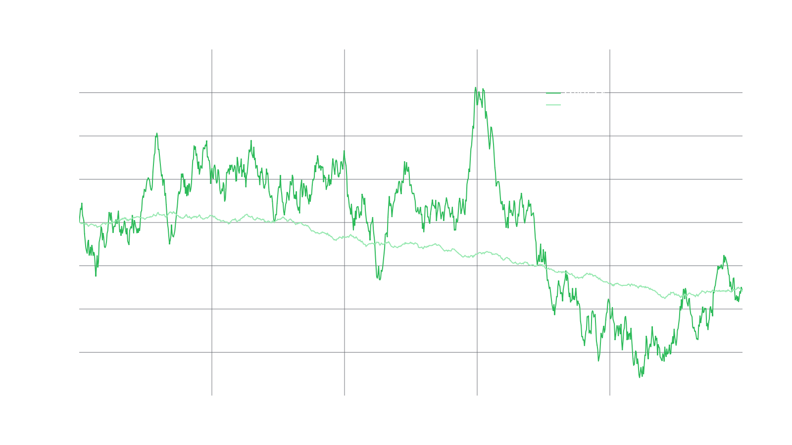
Taking the intuition from the previous example, let's look at the graph below where we visualize two price paths with the same beginning and end price but with drastically different volatility and recorded prices along the way. Note as well that both paths have the exact same number of trades. The price path of "High IV" would produce far more fee revenue for LPs than the "Low IV" path even though the portfolio value would be the same for the LP at the beginning and end (time $t=0$ and time $t=1$ respectively)! The reason the "High IV" path earns more is that the price changes are larger and, for a CFMM, this means the swap volume is larger. Again, this higher volume yields higher fees. We can also see that volatility and volume have an intimate relationship in CFMMs.

Liquidity Distribution Implications

Path dependence has significant implications on the optimal liquidity distribution in CFMMs. As fees are directly related to the price path, it becomes crucial for liquidity providers to strategically distribute their liquidity across anticipated price ranges to maximize their returns. By understanding the potential price paths and market dynamics, LPs can better position themselves to capitalize on price fluctuations and collect more fees.

In the first scenario the optimal price range would be to distribute all the liquidity between the prices of $P_{start}$ and $P_{end}$. In the second scenario, the optimal distribution would depend on the intermediate prices as well. For example if $P_1<P_{start}$, than the optimal distribution would be between $P_1$ and $P_{end}$. In hindsight it is much simpler to pick out the ideal distribution, however in practice, it is not so simple without foresight into the price path of the asset pair.

In practice, The less prices being allocated to for a volatile price pair, the more frequently the user will have to change positions in order to continue earning fees. This means that LPs should consider diversifying their liquidity allocation and not solely focus on a narrow price range. By spreading their liquidity across various price levels, they can benefit from multiple price paths and enhance their fee-earning potential. An obvious exception to this would be with stable token pairs such as ETH-stETH and USDC-DAI and other assets expressing mean reversion in price.

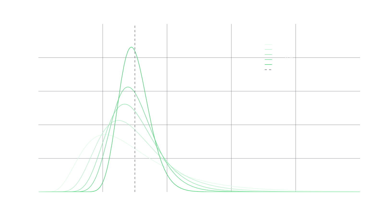
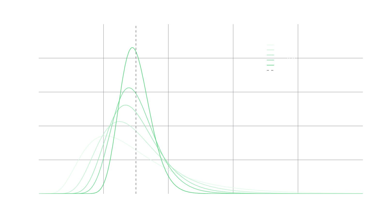
An advantage of CFMMs as a market structure is they can be used to express a majority of these desired liquidity distributions passively. This actually even extends to being able to express dynamic liquidity distributions as well (meaning distributions that change over time). An example of this would be the RMM-CC curve, which expresses a log-normal distribution that converges with an expiry at a single strike price, as shown in the graph below. This effectively allows users to express more complex views on the market while still remaining as passive as possible.

Connecting Path Dependency and Fee Growth

As illustrated earlier, path dependence plays a significant role in determining fee growth in a CFMM. Since fees are generated based on swap volume and the associated price changes, different price paths can lead to different fee outcomes for LPs. This also highlights the importance of liquidity distribution in maximizing fee growth.

As discussed in the previous subsection, a well-distributed liquidity pool can allow larger swap volumes and reduce slippage, in turn boosting fee growth. Conversely, a badly distributed liquidity pool could lead to smaller swap volumes and higher slippage, reducing fee income. This is because the liquidity distribution is directly tied to the market depth, which indicates the expected volume for a given price change.

Understanding the connection between path dependence, liquidity distribution, and fee growth can help LPs make more informed decisions about allocating their assets in a CFMM. By considering the potential price paths, liquidity distributions, and the associated market depths, LPs can better anticipate the risks and rewards of their liquidity provision and adjust their strategies accordingly.

In short, path dependence, liquidity distribution, and fee growth are interconnected aspects of a CFMM. By recognizing these relationships, LPs can optimize their asset allocation to maximize returns and minimize risks in changing market conditions.

Dynamic Allocation

Now that we know how fee growth is affected by path dependency on price, we can discuss the implications it has on allocation decision-making. For this section we are going to assume the goal of the LP isn't to replicate a specific portfolio using LPTs, but instead is simply to maximize fee income earned.

The most fees are earned when all of your liquidity is underlying the current global price for the pair. This is because if the global price changes slightly, an arbitrageur would have to swap all of your liquidity in terms of swap volume just to move the price away from its current state, meaning you earn the fee off your entire liquidity. In a sense, this says the goal of our allocation should be to track the price path using our liquidity distribution.

Dynamic allocation in our context involves rebalancing the distribution of assets held in CFMM position based on the observed price paths, trading volumes, and liquidity demands. By actively monitoring and updating their pool allocations, LPs can optimize their positions to maximize the fees earned. The rebalance events made during dynamic allocation are crucial to maximizing fee growth. Without complete knowledge of the future price path, it will be extremely hard to damn near impossible to optimally allocate a single time without the need for rebalance ever. In a sense, maximizing fee growth in the long term requires you to be a more active provider rather than a purely passive user.

Leveraging RMMs

While being an active LP is essential for maximizing fee growth, it is worth noting that CFMMs, and more specifically, RMMs can be utilized to replicate more dynamic distributions. This allows users to maintain a relatively passive approach without missing out on additional fee income.

For example, the RMM-CC curve, as mentioned earlier in the article, expresses a log-normal distribution that converges with an expiry at a single strike price. By leveraging RMMs with dynamic distributions, LPs can create positions that adjust their liquidity distributions over time. These dynamic distributions enable users to express more complex market views while still remaining as passive as possible. This way, LPs can benefit from the potential fee growth associated with active management while minimizing the cost incurred to constantly monitor and rebalance their positions.

The combination of active monitoring and leveraging RMMs for dynamic distributions can help LPs maximize their fee growth while still maintaining a relatively passive approach. Understanding these concepts and their interplay is crucial for making informed decisions about asset allocation in CFMMs and adapting to ever-changing market conditions.