Portfolio Management: Value Functions and LP Shares

Liquidity Provisioning
When allocating assets to an Automated Market Maker (AMM), the user will gain exposure to a unique portfolio of tokens. As the prices of these tokens change over time, the autonomous nature of AMMs will cause the depositor's portfolio to be altered. This presents a compelling use case for depositors to use AMMs to design portfolios of their own choosing that fit their changing opinions over time. Decentralized Finance (DeFi), enables AMM technology in a permissionless and trustless way. The autonomous nature of DeFi gives Liquidity Providers (LPs) for AMMs unique portfolio management abilities and opportunities. One such example is that LPs no longer have a need for a direct counterparty or manual rebalancing through onchain trades, though the latter can be improved nicely as well. AMMs are able to remove the need of counterparties by incentivizing other specialized parties called arbitrageurs instead. These arbitrageur agents actively trade on the LP's behalf in order to let an LP achieve their desired portfolio composition. Let's dive in.
Portfolio Value
Suppose that an LP deposits into a pool containing two different assets: Token and Token . Getting the value of their share relies on knowing the both the amount of each asset as well as their current prices.
To keep this material concrete, we should think of Token as and Token as which we will also denominate prices in. At any given time, an LP share will consist of some amount of reserves of Token and of Token . If the price of Token in terms of Token is , then the value of the LP share is given by the following formula: In AMMs, a changing price will change and , so in general the portfolio value is a function of price: We will refer to as the _portfolio value function (PVF)*. Understanding the PVF of various AMM positions is essential for LPs who wish to manage their portfolio in a multitude of ways.
At Primitive, we work with Constant Function Market Makers (CFMMs) which are a type of AMM that use predetermined mathematical functions to set prices, manage liquidity, and facilitate swaps. When LPs deposit funds into CFMMs, they will take on an assumed PVF that we can calculate explicitly ahead of time. As further compensation, LPs may also earn fees on swaps that go through the CFMM they are providing liquidity to, but this cannot be calculated ahead of time due to the inherent randomness of price fluctuations. Due to arbitrageurs taking advantage of the deterministic nature of CFMMs, fees are included on all swaps against a pool to reward LPs and these fees can be re-invested into the pool as additional liquidity.
Hence, LPs must consider both PVFs as well as fee generation when deciding to allocate into LP shares. In this piece, we will focus on the first perspective of PVFs and decouple the notion from fees. Fees, volume, and volatility will be left for a subsquent article.
Replicating Market Makers
CFMMs are built solely on a trading function which tells us how to compute the reserves that make up an LP share for any given price as well as determine an associated PVF. This relationship is important, but it would be nice if a depositor who has a target portfolio outlook could instead choose some PVF of their own and define a trading function from there. As a result, the depositor could speculate on the future, decide upon their target portfolio allocation, and deposit into a handful of CFMMs to achieve their objective.
Fortunately, the conversion from a chosen PVF to a unique trading function is provided by the paper "Replicating Market Makers (RMMs)". In the paper, the authors suggest that a CFMM's trading function can be viewed as a means to construct a "replicating" portfolio. Specifically, a CFMM's trading function is a means to programmatically achieve a target PVF. Formally, the RMM paper gives an algorithm to get CFMM trading functions from a certain class of PVFs that are: non-negative, non-decreasing, and concave.
Leverage and Exposure
A depositor has at least two quantities to balance in their mind: capital growth and risk. Naively, if the depositor believes the price of will increase, the depositor can enter a long position by purchasing an amount of and holding on to this until satisfied. For clarity, assume that the depositor has enough capital to purchase exactly one Token as they create their position. Using our formula from before, the depositor in a long position experiences a PVF of :
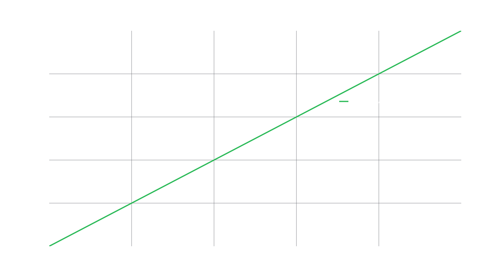
The trader is exposed to equal upward and downward movements in price meaning that their portfolio's value changes one-to-one with the volatility of too. If the depositor exudes confidence in the performance of Token , they may wish to gain additional leverage on the asset and if the trader is less confident, they may want to reduce their leverage. The latter case is quite simple, just have the trader purchase less than one Token , whereas the former requires more machinery around accruing additional exposure with their given collateral. Nonetheless, the amount of leverage in the PVF will land the trader somewhere in the graph below:
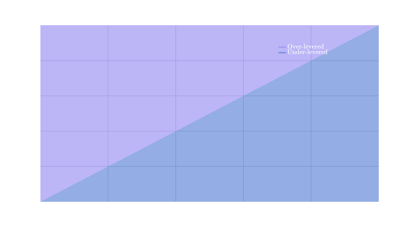
CFMMs cannot list negative prices and depositors in CFMMs cannot take on negative balances or hold negative shares natively. This tells us that is a non-negative function. All we will need to do for CFMMs is stay within this quadrant we have graphed here. The only means in which the PVF can ever decrease is if the depositor can hold negative shares, i.e., a short position. Since basic CFMMs do not allow for this, the PVF must also never decrease. For all intents and purposes, it must be that the PVF has zero value when Token has zero value unless we also take time-variance and fees into account since the depositor cannot create captial from nowhere.
Concavity
Not all PVFs are straight lines. For instance, if a depositor's PVF curves downward (but does not decrease!) into the "Under-levered" region, then the depositor has effectively sold some of their share of Token along the way. This reduces some risk the depositor has by cashing out as the price increases. If a depositor's PVF enters into the "Over-levered" region, then it is as if the depositor has purchased more of Token than their original capital would let them. You may now see why producing over-leveraged positions is difficult yet beneficial for the extremely confident (and risk inclined) depositor. These examples are getting at the idea of dynamically altering the leverage of a PVF with respect to price. This leads us into the notions of concavity and convexity which refer to the second derivative with respect to price of the PVF (often called the Greek "Gamma").
Suppose that the depositor believes that as the price of increases, that the depositor wishes to reduce their exposure to or sell off as the price increases. This can be done to reduce their risk or collect profit. If the price drops, they may also wish to acquire more of the asset in hopes to sell off at higher prices. One such PVF that accomplishes this goal is the PVF . This, coincidently, is the payoff function of the constant product market maker which is used by Uniswap. This PVF looks like:
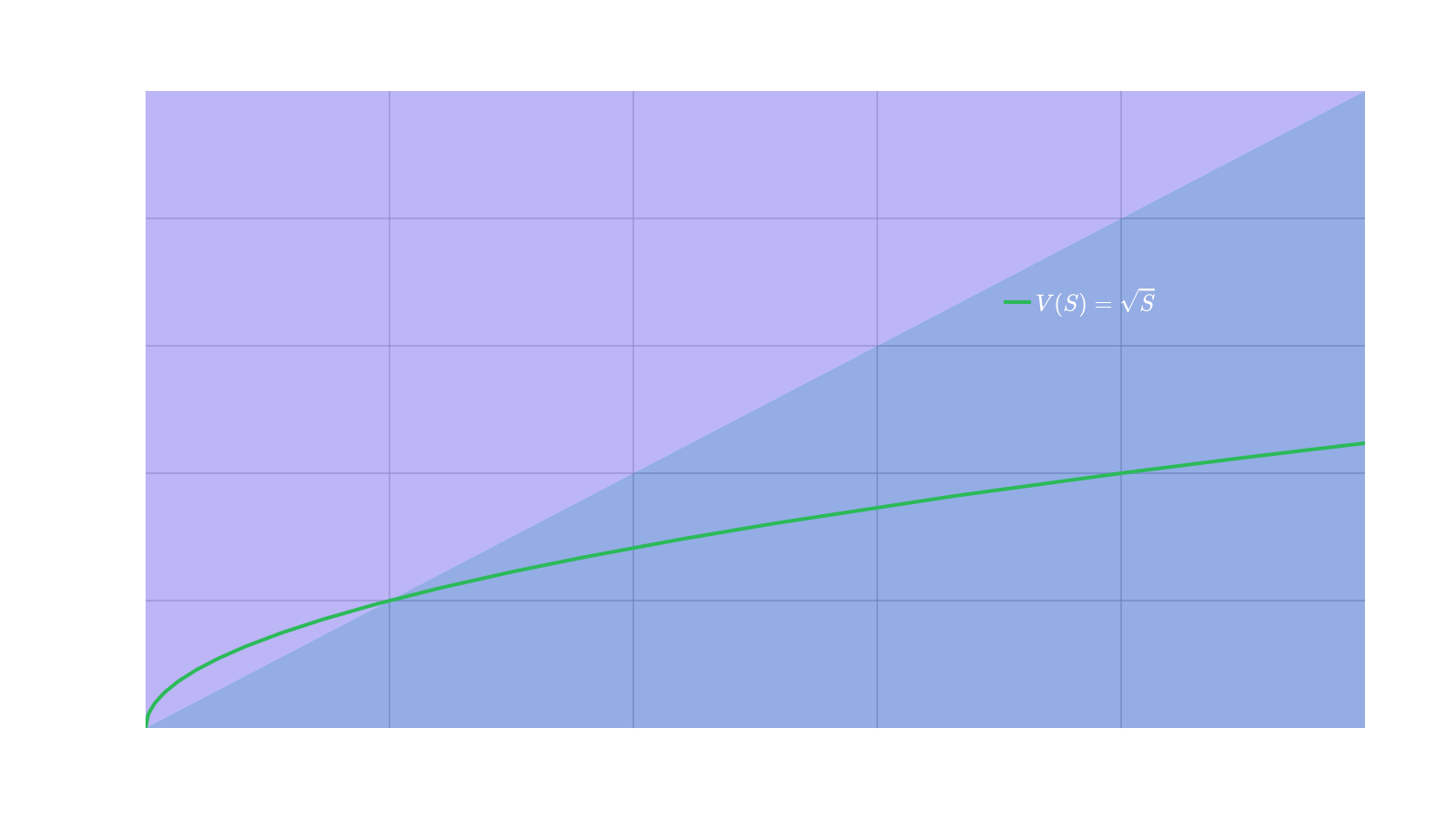
Since the depositor commits to selling as the price increases, their PVF necessarily curves downward. This is referred to as concavity. One may also notice that this can dampen the effects of the volatility of on the PVF. The mechanics of CFMMs is exactly the same as the goal of the trader who sells as the price increases. This tells us that a CFMM will always have a PVF that is a concave function. Reflecting momentarily, we have described exactly the range of shapes that a CFMM PVF can have just from first principles. It is this intuition that guided the authors of the RMM paper to search for a way to define a trading function from a PVF.
Convexity
On the other hand, if the depositor is to become even more confident in as its price increases, then the trader would like to increase their leverage in higher price ranges. Graphically, this would lead to their PVF curving upward. However, to do this, the depositor must do something akin to purchasing more as the price climbs higher. An example of a PVF that accomplishes this payoff is which looks like:
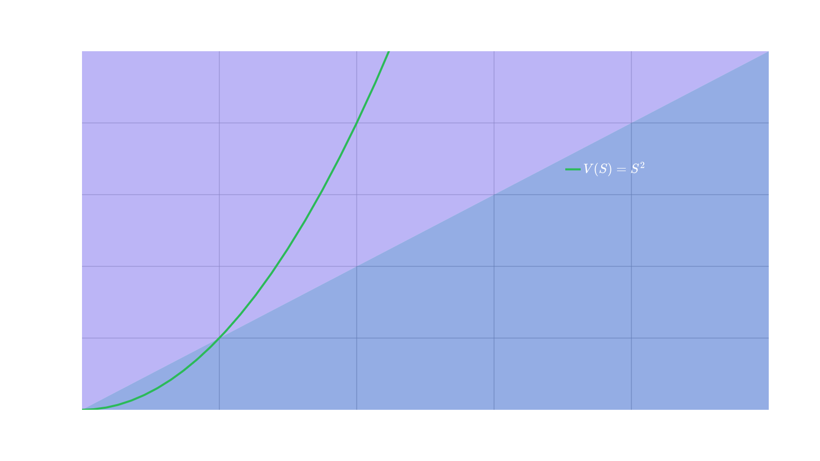
Of course, this perspective can be quite risky! But, it has a different risk profile than a linear PVF that is over-levered. In fact, as the price dips below one, the PVF is underlevered. Convexity can be an excellent tool as you gain the benefit of increased leverage as price increases and decreased leverage as price decreases. Further, convex PVFs are a reason why call options can be popular in bull markets.
The process of increasing leverage through convexity hints at the need for another mechanism alongside CFMMs since there needs to be a way to effectively purchase as price increases. This exact topic goes beyond the content of this post, but there are a handful of sources . Briefly, one may notice that the concave and convex PVFs given before are inverse to one another. More generally, this fact tells us that by borrowing and lending LP shares we can produce a convex PVF.
Diversification
As a depositor considers the broader market, they may construct multiple strategies for a given pair of tokens or even construct strategies on a larger basket of tokens. Given that, they may also wish to be an LP in a multitude of different pools. In Portfolio, pools consist of pairs of tokens and each can have its own unique PVF. The fortunate property of PVFs is that they can be combined together nicely. For instance, if a depositor deposits half of their capital into Pool 1 and half of their capital into Pool 2, then their accumulated PVF is just the sum of the individual PVFs. This gives us a resultant PVF for their portfolio that is diversified across two different pools for the same token pair. Nothing changes if the second pool consists of different tokens aside from the equations looking messier.
With enough variety of pools and token pairs, PVFs can be tailored to fine grain precision for a depositor. Given that each PVF comes from a CFMM pool, the accumulated PVF will still be non-negative, non-decreasing, and concave without additional mechanisms. However, this gives a large landscape of positions to choose from in order to construct the ideal PVF for their beliefs.
Adjusting Over Time
As time moves forward, the depositor must be willing to change their perspective on their positions or else they can increase risk. In order to provide this type of service, the depositor must either move positions entirely and manually or they can instead change the CFMM trading function over time programmatically. Actually, the purpose of the Financial Virtual Machine is to make the former process cheaper and easier. In the latter case, programmatic time-variance allows a depositor to not only diversify, but also to implement forecasts. Let's finish with a more involved PVF which comes from a CFMM that we call RMM-CC which accomplishes the goal of constructinga time-varying payoff.
Suppose the depositor wishes to choose an expiry date in the future for which they are willing to either buy or sell Token at some final price . However, the further away from expiry the depositor is, the less they are willing to hold Token . This displays increasing confidence in the performance of in the future compared to the current time. If this is the case, then the the depositor can diversify into an RMM-CC position to achieve this type of objective. Also, the depositor may wish to have their rate of confidence increase differently over time compared to others, so they add an additional parameter to dictate how rapidly they wish to increase their belief of the value of Token . All in all, the PVF over time for some choice of parameters would look as follows:
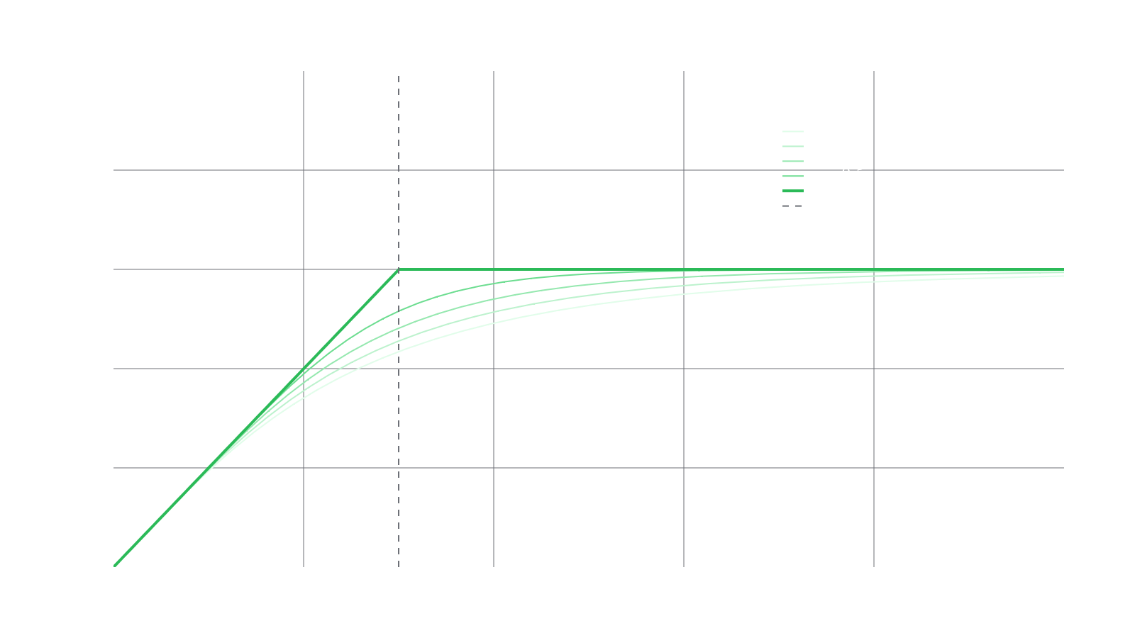
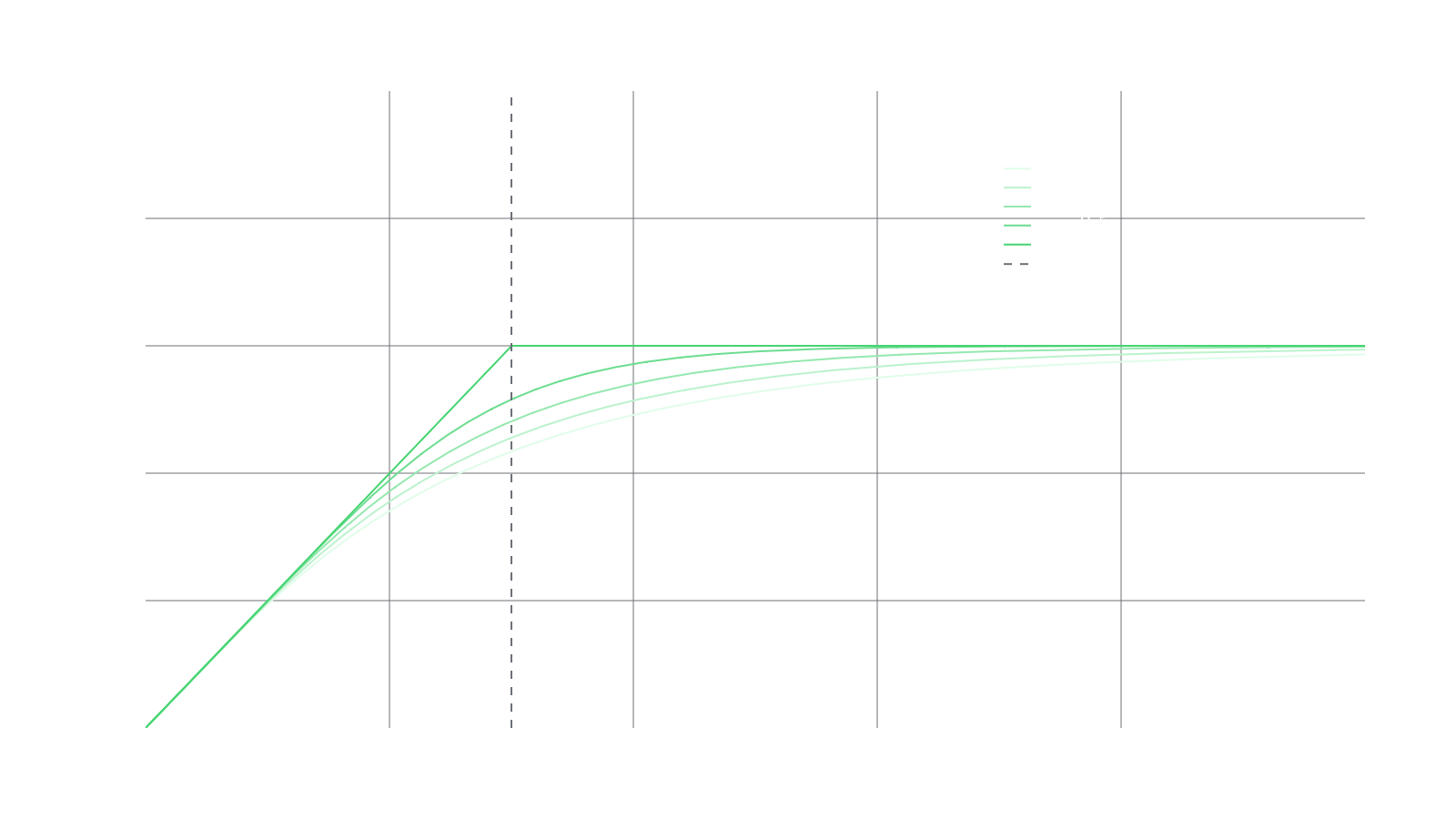
The goal of creating RMM-CC was to mimic the value of a Black-Scholes covered call over time. This means that the PVF depends on both price and time so we put . Ignoring fees or premium, is always underleveraged and furthermore, where is the user-defined final price of the pool. The final price of the pool is reached at a time and the time til expiry . One final parameter is which dictates how swiftly the PVF will change over time. The PVF for RMM-CC with , and over various 's is:
Further Remarks
Portfolio value functions are one aspect that help investors understand the risks and rewards associated with different LP positions. With a solid grasp, PVFs can be tailored for very specific outlooks and risk profiles. However, it is not the only aspect to constructing a portfolio of tokens and we will discuss other aspects in future content.
- The RMM paper by Guillermo Angeris, Tarun Chitra, and Alex Evans can be found here: https://arxiv.org/abs/2103.14769.
- The paper by Estelle Sterrett, Waylon Jepsen, and Evan Kim called "Replicating Portfolios: Constructing Permissionless Derivatives" shows how a depositor can use borrowing and lending techniques alongside LP positions to create other structured products. It can be found here.