Gamma Exposure for Liquidity Providers Leads to Loss-Versus-Rebalancing

Introduction

In Traditional Finance (TradFi), Market Makers (MMs) constantly hedge their Gamma Exposure (GEX) to avoid losses. As a Liquidity Provider (LP) in Decentralized Finance (DeFi), unlike a MM in TradFi, your position is constant, and there is no way to hedge GEX without using other instruments. The inability to hedge GEX causes LPs to lose profits by Loss-Versus-Rebalancing (LVR).

TradFi MM Risk

Options Delta and Gamma

Put and call options are agreements between two parties on selling or buying assets for a specific price on a certain date. As a trader, options allow for more fine-grained control over payoffs and can cap downside risk because options have nonlinear payoffs, unlike longs or shorts on the underlying asset. The nonlinear payoff allows traders to make directional bets and hedge unfavorable price movements.

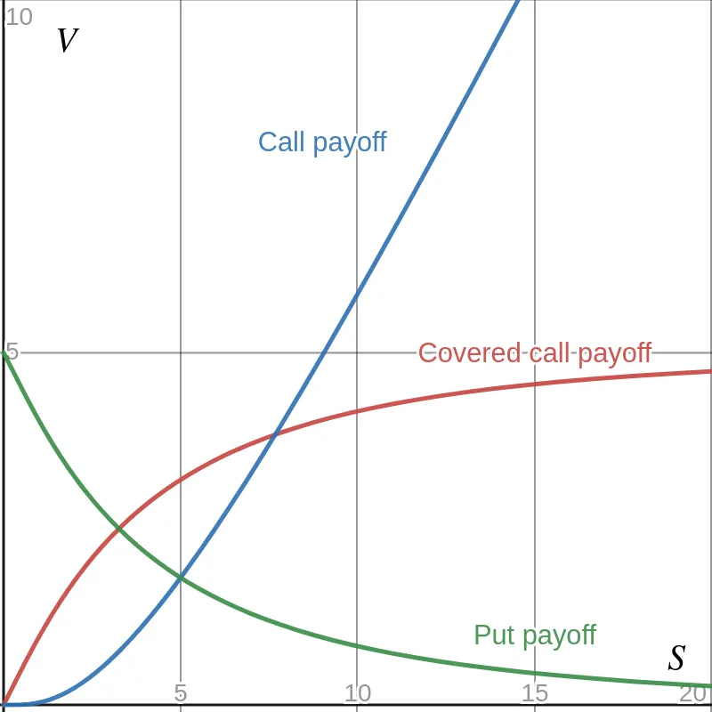
Look at the payoff curves for a put, a call, and a covered call. Pick a point on one of the curves. At the chosen point, the curvature (really, the second derivative) is referred to as the Greek letter Gamma $\Gamma$. The call and put both have positive $\Gamma$, and the covered call has negative $\Gamma$.

For some prices $S$, the curves may have larger curvature, which means the magnitude of $\Gamma$ is larger. Along any of the mentioned payoff curves, the slope of the line tangent to the curve at a price is the option’s Delta $\Delta$ (another Greek letter).

Notice that both a call and covered call have positive slopes for all prices, therefore positive $\Delta$. In contrast, the put has negative $\Delta$.

The preceding logic tells us that $\Gamma$ is the rate of change in $\Delta$! The formal relationship between $\Gamma$ and $\Delta$ is calculus-based and codified by the Black-Scholes equation. Succinctly, if $V(S)$ is the value of some position for price $S$, then $\Delta=V’$ and $\Gamma=V’’=\Delta’$.

Gamma Exposure

In TradFi, MMs commonly play the role of a counterparty for options sales. However, an MM is not interested in making directional bets on any asset. Let’s explore the problem that arises from MMs’ indifference to directional bets through an example:

Suppose a trader wants to purchase a call with $\Delta=20$. So long as the bid for the option fits the set bid/ask spread provided by the MM, the MM sells the option to the trader. Thus, the MM is short a call and has exposure to $\Delta=-20$.

To hedge this $\Delta$ risk, the MM buys 20 shares of the underlying asset to get zero $\Delta$ on their position since each share has $\Delta=1$. But, since a long position on the asset has zero $\Gamma$, the MM now has nonzero $\Gamma$ exposure, and they must actively manage their long position to maintain $\Delta$-neutrality.

In the example, MMs are required to actively manage their position to mitigate their GEX. GEX can be positive or negative depending on the options flow at a given price. If an MM was not active, a movement in the price for the underlying would lead to a nonzero delta which is not ideal.

Now, imagine a scenario where an MM is long or short many different puts or calls of various strike prices and expirations. In this case, their GEX varies from price to price and dictates the MM’s choice to take on more longs or shorts. There is some ability to predict the movement and volatility of the market price given the MM’s desire to remain $\Delta$-neutral. For more on TradFi MM GEX, see the GEX whitepaper.

DeFi LP Risk

Loss-Versus-Rebalancing for Liquidity Providers

In the paper Automated Market Making and Loss-Versus-Rebalancing (preprint), the authors Milionis et al. seek to characterize Impermanent Loss (IL). More truthfully, they define a general measure of Loss-Versus-Rebalancing (LVR), which allows the LP to choose their own benchmark for portfolio balancing. For example, when the benchmark is to HODL, meaning there is no rebalancing and we are comparing against the performance of buying and holding the underlying, the loss an LP experiences is IL. After a handful of assumptions about the price process, the authors find that the instantaneous LVR, pronounced “lever,” assumes the form:

To get the total LVR, just add up the instantaneous LVR over the path the price follows in time. In the above equation, note that $\sigma$ is the market volatility and that $V’’(S)$ is precisely the $\Gamma$ of the LP’s position.

How can we think of this quantity? Milionis et al. prove in Proposition 1 that LVR is equivalent to the profit earned by arbitrageurs, and the profit for arbitrageurs is profit that the LPs cannot capture! Thus, by managing an LP’s GEX, the LP can take back profit from arbitrageurs and keep it for themselves.

Milionis et al. then define Loss-Versus-Holding (LVH), which is the exact definition of impermanent loss:

For LPs, we see that LVH is given by taking $x_s=x_0$, and they show that LVH has variation bounded below by LVR.

What’s the point of all of this? Mainly, at any moment with a priori known market volatility, the current price and LP GEX at that price determine LVR (or LVH). In this sense, LPs lose profit due to their inherent GEX and inability to actively hedge it.

Replicating Monotonic Payoffs

LVR was hinted at in an earlier paper Replicating Monotonic Payoffs Without Oracles (preprint). The authors Angeris et al. argue that the quantity W below represents the total arbitrageur profit.

Notice the term in the integrand $g(S)$. Using their Eqn. (4):

We can realize $V’(S)=g(S)=x^*(S)$. Note that $W$ is defined for any price process. Suppose we assume the same price process as Milionis et al. (Geometric Brownian Motion). It is a matter of applying Ito’s lemma, as in the proof of Theorem 1 of the paper by Milionis et al., to see that this integral from the Monotonic Payoffs paper is LVR.

For Researchers

Given that an LP experiences losses due to the inability to hedge GEX actively, it is of great interest to design LP positions that allow for active liquidity management. One example is dAMMOp. Proper active management would mitigate GEX. Furthermore, the original purpose of the GEX whitepaper was to use MM GEX as a proxy for market volatility.

For CFMMs, computing the LP GEX is not too difficult, and the cumulative GEX for DEXs could prove to be an interesting means for constructing a decentralized volatility oracle. If we also knew that some LP positions were using borrowed assets, this would imply opposite GEX for those positions and bring liquidations into the mix. Can we quantify the GEX for DEXs that are combined with borrowing/lending protocols?

The Primitive team studies market design and MEV in the DeFi space. We value education, free information and sovereignty. Our research emphasizes improved UX for DeFi. Follow us on Twitter and see our GitHub for open source code and docs.