Primitive Arbitrage

Waylon Jepsen

Waylon Jepsen

September 16, 2022

Constant Function Market Makers

CFMMs are the dominant design architecture of decentralized exchanges (DEXs). CFMMs are commonly implemented as a standalone piece of software that acts as a trusted third party. Trades are automatically facilitated against the reserves of tokens held in a CFMM. Any actor can add or remove liquidity to the reserves during the lifetime of a pool to participate in making the market. Actors are incentivized to add liquidity to the reserves because they earn swap fees denoted by gamma laying within the interval zero (exclusive) to one (inclusive). The available actions to interact with a CFMM are determined by its trading function. Formally, a CFMM is an $n$ -token pool of positive real numbers and a trading function such that

\varphi: \mathbb{R}^n_+ \rightarrow \mathbb{R}

Given any $\mathbb{R}$ , the value the trading function $\varphi$ evaluates to is called the invariant. The quantity of reserves of an $\textsf{Token}_i$ of an $n$ -asset pool is denoted $R_i$ where for every $i\in\{1,…,n\}$ where $i$ specifies a specific asset. Reserves change when trades are executed. For example in the ETH/USDC liquidity pool $\textsf{asset}_1 =$ ETH, and $\textsf{asset}_2 =$ USDC, $R_1$ denotes the quantity of ETH in the pool and $R_2$ denotes the quantity of USDC respectfully.

Exchange Rate

Recall that a trading function is a function of asset reserves. The trading function determines the exchange rate of assets in a CFMM. Since trades change the reserves, and the exchange rate is in terms of the trading function, trades can also impact the price. The price denotes the value of one asset in terms of another. Because you can’t ensure that your trade is executed at an exact price and that there may be some trade before you in the current block, you must allow some price tolerance such that as long as that price deviates within this bound, your trade will still go through. This tolerance is called slippage and is proportional to the price impact of your trade. Given a CFMM the price vector is

\mathbf{P}\coloneqq \nabla \varphi

and the reported price of $\textsf{Token}_i$ is

p_i := \frac{P_i}{P_n}

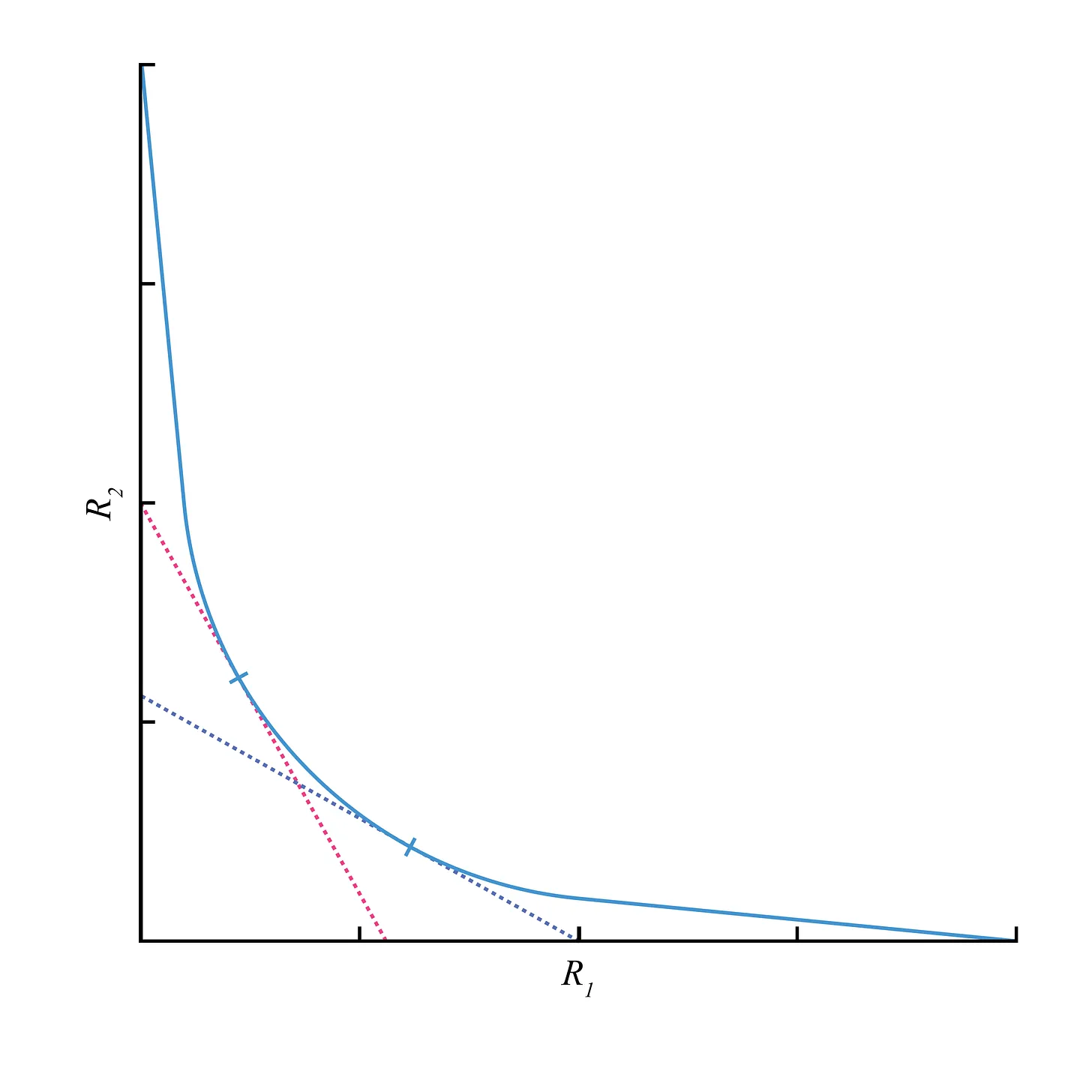
Recall that the gradient $\nabla$ is a vector of derivatives. The price $p_i$ is the derivative of the trading function with respect to $\textsf{Token}_i$ over the derivative of the trading function with respect to $\textsf{Token}_n$ . The exchange rate graphically corresponds to the tangent line at a point on the trading function. The slope of this tangent line is the additive inverse of the exchange rate and can be seen for two different measures of reserves in the graph below.

Price Impact and Arbitrage

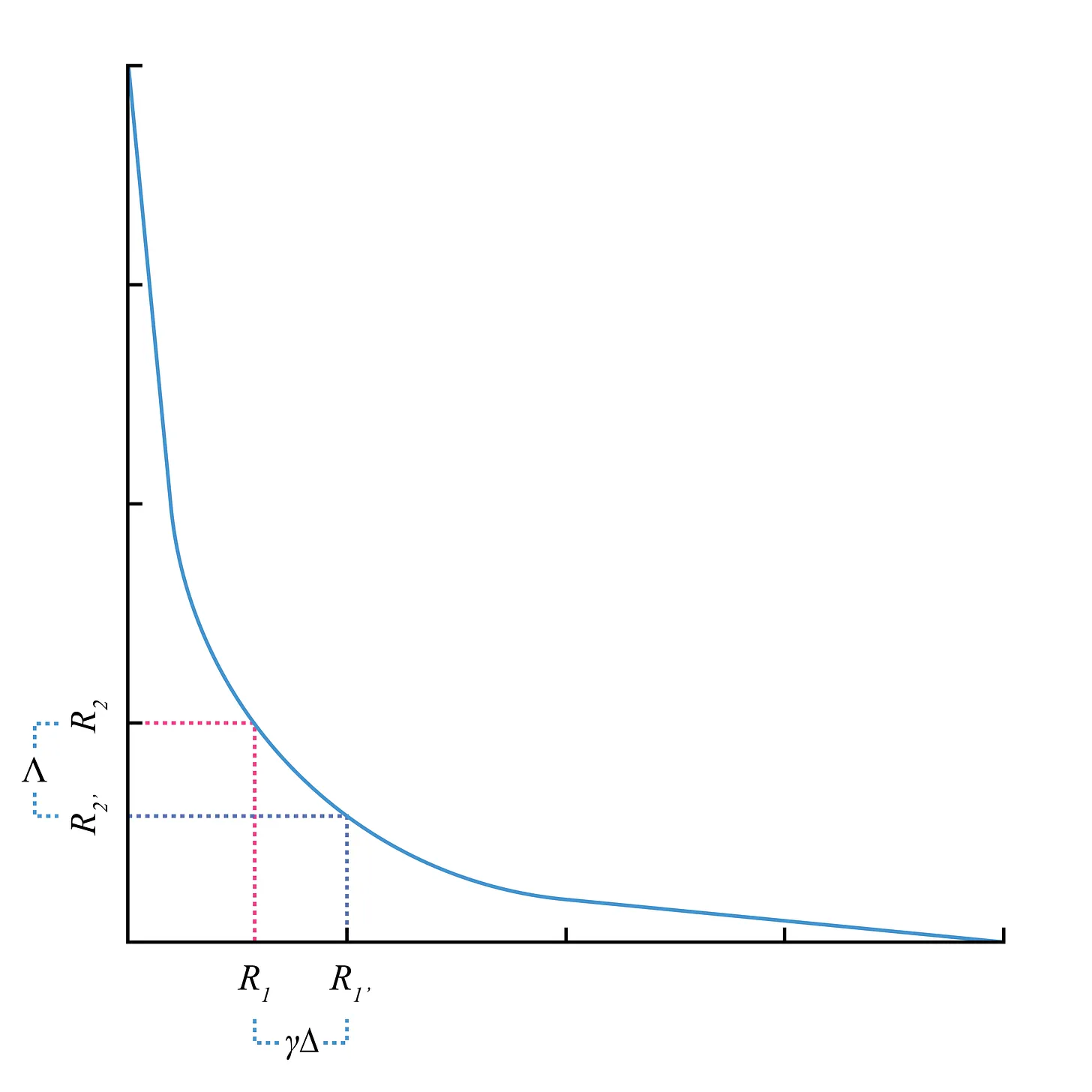
Recall that all trades on a CFMM have a price impact, thought of as the change in price for a given trading function $\varphi$ . If there is a high demand for $\textsf{Token}_1$ the reserves of $\textsf{Token}_2$ in the CFMM will diminish, and the trading function will price this token higher. How can we ensure that the price is aligned with the greater market? Arbitrage is when an actor is aware of a price discrepancy between marketplaces and executes a series of trades to exploit this discrepancy. All markets for a given asset pair tend to converge on an expected price due to arbitrage. To perform this arbitrage optimally (i.e., maximizing profit), the arbitrageur needs to know the exact size of their arbitrage trade that will align the price. A given price impact implies a distinct trade size on CFMMs and thus an optimal arbitrage trade quantity exists. Consider a two-asset liquidity pool with assets 1 and 2. The geometric representation of price impact can be seen below as the difference in slope of the tangent lines where $\Delta$ represents the number of assets tendered to the liquidity pool, $\Lambda$ represents the number of assets received from the liquidity pool, and $\gamma$ is the swap fee.

To calculate the required trades for arbitrage, arbitrageurs seek to answer the question: How large does trade have to be to change the price by a certain amount? This question can be thought of as: What is the optimal size of the arbitrage trade such that after the trade, the price is aligned with an external reference market thus, maximizing revenue from the arbitrage opportunity? This was shown for UniswapV2's trading function in the appendix of the Analysis of Uniswap markets paper. In the remainder of this article, we will show this for the trading function of Primitive's RMM-01 trading function.

RMM-01

RMM-01 is a constant function automated market maker (CFMM) deployed by Primitive. RMM-01 approximates the payoff of a covered call to liquidity providers through the aggregation of swap fees. To do this, the curvature of the level sets of the trading function used by the RMM-01 trading function changes over time. RMM-01 follows Black-Scholes option pricing, which requires setting $K$ , $\sigma$ , and $\tau$ parameters at pool creation. For an arbitrageur to maximize their profits and achieve a price equilibrium between two markets, they need to know the exact size of their arbitrage trade corresponding to the optimal arbitrage. Here we refer to this as $\delta$ . To understand the derivation of the optimal arbitrage $\Delta$ for an RMM-01 pool, it is necessary to first examine the RMM-01 trading function. Unlike the static trading function of Uniswap, RMM-01 is a dynamic curve and thus changes over time. The trading function is

\varphi(R_1, R_2) = R_2 - K \Phi(\Phi^{-1}(1-R_1) - \sigma \sqrt{\tau})

Where $\Phi$ is the zero-mean unit-variance Gaussian cumulative distribution function (CDF), $R_1$ is the reserve of the risky asset (ETH), $R_2$ is the reserves of numeraire (USDC), and σ and τ here are the volatility and time to expiry. All the pools in RMM-01 have these parameters and, all the results here can be calculated from onchain information. RMM-01 is normalized per-liquidity provider tokens(LPTs) token, and all solutions here are per LPT. This is not a problem in practice because the quantity of LPTs is also kept onchain and is publicly available.

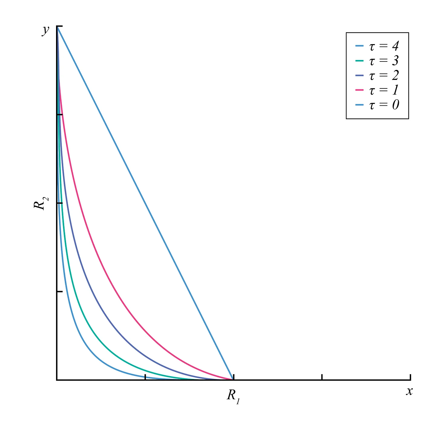
A key property of the trading function is that it is dynamic with respect to $\sigma$ and $\tau$ . Notice at expiry, when $\tau=0$ , the trading function has a constant price at the strike price $K$ , which is graphically interpreted as a straight line with no curvature. We can see the curvature of the RMM-01 trading function in the graph below, where $y$ is the strike price.

Optimal Arbitrage Problem

Consider an RMM-01 ETH-USDC pool and an external reference market where the price of ETH is $(1+\epsilon)p$ where $p$ is the reported price of RMM-01. What is the quantity of ETH we need to tender to RMM-01 for it to match the reference price? Or in other words, what is the precise size of our arbitrage trade that maximizes our profit? We will first calculate the exchange rate of USDC/ETH on RMM-01 using the methods mentioned in the section on the exchange rate. Then we will calculate a new price in terms of some tendered quantity of assets and then invert that function to get the tendered assets in terms of some market price.

Recall that for CFMMs the price of asset $i$ in terms of asset $n$ is $p_i\coloneqq P_i/P_n$ where $\mathbf{P}$ is the gradient vector of the trading function. Taking the derivative of the trading function with respect to $R_1$ gives us

p_1 = Ke^{\Phi^{-1}(1-R_1)\sigma \sqrt{\tau} - \frac{1}{2}\sigma^2\tau}

and the derivative of the trading function with respect to $R_2$ is $p_2=1$ and thus the price of ETH with respect to USDC on RMM-01 is $p_1/1 = p_1$ from above.

Let $g(\Delta_1,0)$ and $g(0, \Delta_2)$ denote the price impacts due to tendering $\Delta_1$ and $\Delta_2$ , respectively. Then if $\Delta_1$ is tendered the price impact is

g(\Delta_1,0) = Ke^{\Phi^{-1}(1-R_1 - \gamma\Delta_1)\sigma \sqrt{\tau} - \frac{1}{2}\sigma^2\tau}

and similarly, if $\Delta_2$ is tendered then the price impact is

g(0,\Delta_2) = Ke^{\Phi^{-1}\left(\frac{R_2 + \gamma \Delta_2}{K}\right)+ \frac{1}{2}\sigma^2\tau}

Solving for $g$ inverse and substituting the desired price change gives the following results. If you want to tender ETH, the optimal size of the arbitrage opportunity is

\Delta_1 = \gamma^{-1}\left(1 - R_i - \Phi\left(\Phi^{-1}(1-R_1) + \frac{\ln{(1+\epsilon)}}{\sigma\sqrt{\tau}}\right)\right)

Interestingly, RMM-01 is not symmetric. This means that if you want to tender USDC, the derivation is different from the solution above and is

\Delta_2 = \gamma^{-1}K\Phi\left(\Phi^{-1}(1-R_1) - \sigma \sqrt{\tau} +\frac{\ln{(1+\epsilon)}}{\sigma\sqrt{\tau}}\right) - \gamma^{-1}R_2

Note that these solutions are per LPT. So say that the market price of an external market for ETH is $2000, and the primitive market price is $1800. Then $\epsilon=0.11111$ and with known values of $\tau$ , $\sigma$ , and $K$ and reserves $R_1$ and $R_2$ , both deltas can be computed trivially and then multiplied by the quantity of LPT tokens.

Conclusion

In this piece, we briefly summarized CFMMs, introduced the dynamic trading function of RMM-01, and presented the optimal arbitrage derivation per LPT value. Searchers are free to compete to capture these arbitrage opportunities. Since the RMM-01 trading function is dynamic concerning στ it is a strong assumption that these arbitrage opportunities will always arise. Thus there will continue to be profitable arbitrage in RMM-01 liquidity pools. The arbitrage not only aligns the price with external marketplaces but also contributes to the payoff of the liquidity providers via the swap fees.