Solstat: A statistical approximation library


Numerical Approximations
There are many useful mathematical functions that engineers use in designing applications. This body of knowledge can be more widely described as approximation theory for which there are many great resources. An example of functions that need approximation and are also particularly useful to us at Primitive are those relating to the Gaussian (or normal) distribution. Gaussians are fundamental to statistics, probability theory, and engineering (e.g., the Central Limit Theorem).
At Primitive, our RMM-01 trading curve relies on the (standard) Gaussian probability density function (PDF) , the cumulative probability distribution (CDF) , and its inverse . These specific functions appear due to how Brownian motion appears in the pricing of Black-Scholes European options. The Black-Scholes model assumes geometric Brownian motion to get a concrete valuation of an option over its maturity.
solstat is a Solidity library that approximates these Gaussian functions. It was built to achieve a high degree of accuracy when computing Gaussian approximations within compute constrained environments on the blockchain. Solstat is open source and available for anyone to use. An interesting use case being showcased by the team at asphodel is for designing drop rates, spawn rates, and statistical distributions that have structured randomness in onchain games.
In the rest of this article we'll dive deep into function approximations, their applications, and methodology.
Approximating Functions on Computers
The first step in evaluating complicated functions with a computer involves determining whether or not the function can be evaluated "directly", i.e. with instructions native to the processing unit. All modern processing units provide basic binary operations of addition (possibly subtraction) and multiplication. In the case of simple functions like where , , and are integers, computing an output can be done efficiently and accurately.
Complex functions like the Gaussian PDF come with their own unique set of challenges. These functions cannot be evaluated directly because computers only have native opcodes or logical circuits/gates that handle simple binary operations such as addition and subtraction. Furthermore, integer types are native to computers since their mapping from bits is canonical, but decimal types are not ubiquitous. There can be no exponential or logarithmic opcodes for classical bit CPUs as they would require infinitely many gates. There is no way to represent arbitrary real numbers without information loss in computer memory.
This begs the question: How can we compute with this restrictive set of tools? Fortunately, this problem is extremely old, dating back to the human desire to compute complicated expressions by hand. After all, the first "computers" were people! Of course, our methodologies have improved drastically over time.
What is the optimal way of evaluating arbitrary functions in this specific environment? Generally, engineers try to balance the "best possible scores" given the computation economy and desired accuracy. If constrained to a fixed amount of numerical precision (e.g., max error of ), what is the least amount of:
- (Storage) How much storage is needed (e.g., to store coefficients)?
- (Computation) How many total clock cycles are available for the processor to perform?
What is the best reasonable approximation for a fixed amount of storage/computational use (e.g., CPU cycles or bits)?
- (Absolute accuracy) Over a given input domain, what is the worst-case in the approximation compared to the actual function?
- (Relative accuracy) Does the approximation perform well over a given input domain relative to the magnitude of the range of our function?
The above questions are essential to consider when working with the Ethereum blockchain. Every computational step that is involved in mutating the machine's state will have an associated gas cost. Furthermore, DeFi protocols expect to be accurate down to the wei, which means practical absolute accuracy down to ETH is of utmost importance. Precision to is near the accuracy of an "atom's atom", so reaching these goals is a unique challenge.
Our Computer's Toolbox
Classical processing units deal with binary information at their core and have basic circuits implemented as logical opcodes. For instance, an add_bits opcode is just a realization of the following digital circuit:

These gates are adders because they define an addition operation over binary numbers. These full adders can be strung together with a carry-out pin for higher adders. For example, a ripple carry adder can be implemented this way, and extended to an arbitrary size, such as the 256bit requirements in Ethereum.
Note that adders introduce an error called overflow. Using add_4bits to add 0001 to 1111, the storage space necessary to hold a large number is exhausted. This case must be handled within the program. Fortunately for Ethereum 256bit numbers, this overflow is far less of an issue due to the magnitude of the numbers expressed (). For perspective, to overflow 256bit addition one would need to add numbers on the order of the estimated number of atoms in the universe (). Furthermore, the community best practices for handling overflows in the EVM are well understood.
At any rate, repeated addition can be used to build multiplication and repeated multiplication to get integer powers. In math/programming terms:
and for powers:
Subtraction and division can also be defined for gate/opcode-level integers. Subtraction has similar overflow issues to addition. Division behaves in a way that returns the quotient and remainder. This can be extended to integer/decimal representations of rational numbers (e.g., fractions) using floating-point or fixed-point libraries like ABDK, and the library in Solmate. Depending on the implementation, division can be more computationally intensive than multiplication.
More Functionality
With extensions of division and multiplication, negative powers can be constructed such that:
None of these abstractions allow computers to express infinite precision with arbitrarily large accuracy. There can never be an exact binary representation of irrational numbers like , , or . Numbers like can be represented precisely in computer algebra systems (CAS), but this is unattainable in the EVM at the moment.
Without computer algebra systems, quick and accurate algorithms for computing approximations of functions like must be developed. Interestingly arises in the infamous approximation from Quake lll, which is an excellent example of an approximation optimization yielding a significant performance improvement.
Rational Approximations
The EVM provides access to addition, multiplication, subtraction, and division operations. With no other special-case assumptions as in the Quake square root algorithm, the best programs on the EVM can do is work directly with sums of rational functions of the form:
The problem is that most functions are not rational functions! EVM programs need a way to determine the coefficients and for a rational approximation. A good analogy can be made to polynomial approximations and power series.
Using our Small Toolbox
When dealing with approximations, an excellent place to start is to ask the following questions: Why is an approximation needed? What existing solutions already exist, and what is the methodology they employ? How many digits of accuracy are needed? The answers to these questions provide solid baseline to formulate approximation specifications.
Transcendental or special functions are analytical functions not expressed by a rational function with finite powers. Some examples of transcendental functions are the exponential function , the inverse logarithm , and exponentiation. However, if the target function being approximated has some nice properties (e.g., it is differentiable), it can be locally approximated with a polynomial. This is seen in the context of Taylor's theorem and more broadly as the Stone-Weierstrass theorem.
Power Series
Polynomials (like below) are a useful theoretical tool that also allow for function approximations.
Only addition, subtraction, and multiplication are needed. There is no need for division implementations on the processor. More generally, an infinite polynomial called a power series can be written by specifying an infinite set of coefficients and combining them as:
A specific way to get a power series approximation for a function around some point is by using Taylor's theorem to define the series by:
Intuitively, the Taylor series approximations are built by constructing the best "tangent polynomial," for example, the 1st order Taylor approximation of is the tangent line approximation to at
For , there is the resulting series
when approximating around .
Since polynomials can locally approximate transcendental functions, the question remains where to center the approximations.
The infinite series is precisely equal to the function , and by truncating the series at some finite value, say , there is a resulting polynomial approximation:
The function can be written by scaling the input and output of by
This demonstrates what various orders of polynomial approximation look like compared to the function itself.
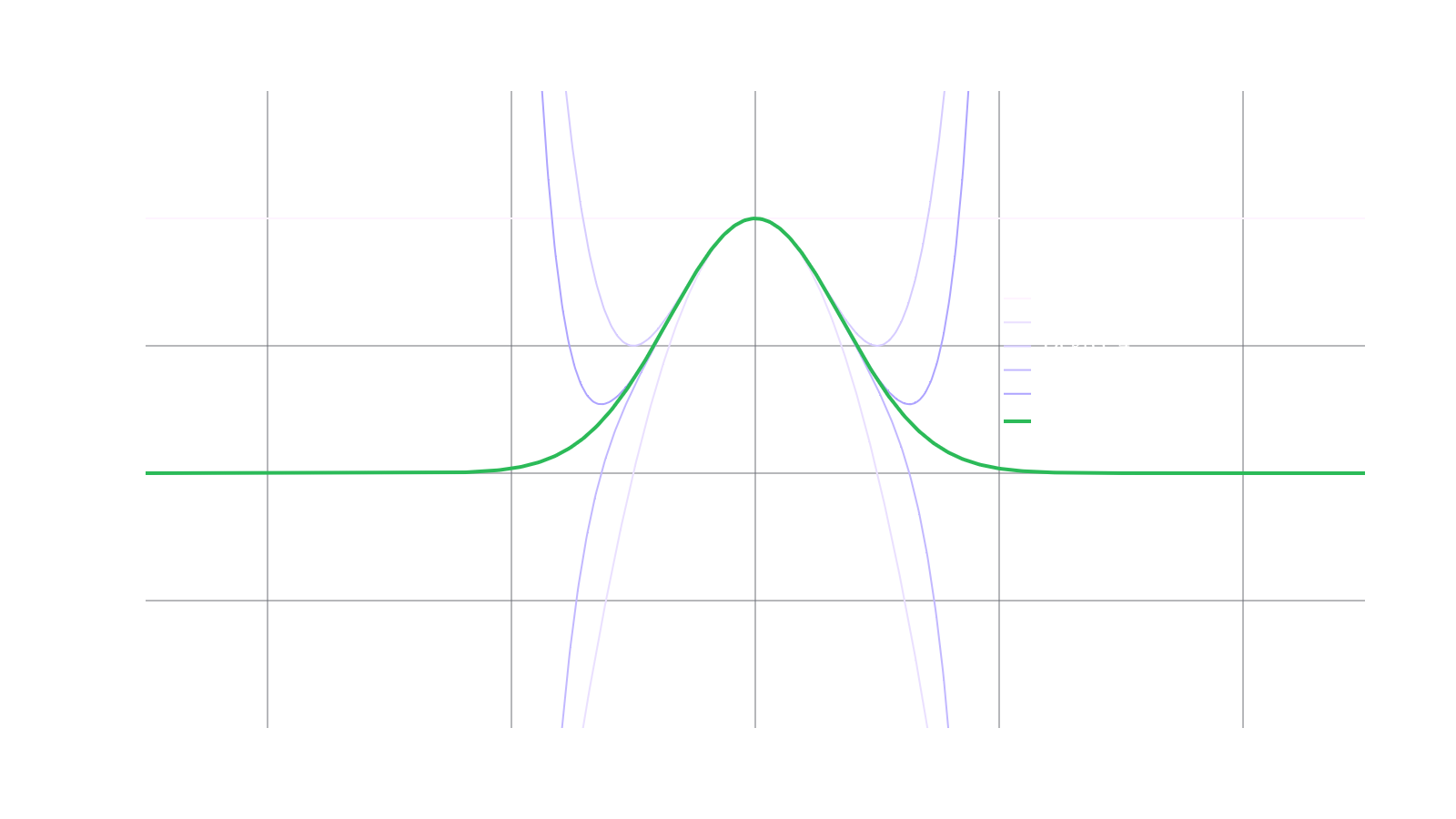
This solves the infinity problem and now these polynomials can be obtained procedurally at least for functions that are times differentiable. In theory the Taylor polynomial can be as accurate as needed. For example, increase . However, there are some restrictions to keep in mind. For instance, since factorials grow exceptionally fast, there may not be enough precision to support numbers like . , so for tokens with 18 digits, the highest order polynomial approximation for on Ethereum can only have degree 19. Furthermore, polynomials have some unique properties:
- (No poles) Polynomials never have vertical asymptotes.
- (Unboundedness) Non-constant polynomials always approach either infinity or negative infinity as .
An excellent example of this failure is the function which asymptotically approaches 0 as . Polynomials don't do well approximating this! In the case of another even simpler function , this function can be approximated by polynomials away from , but doing so is a bit tedious. Why do this when division can be used to compute ? It's more expensive and decentralized application developers must be frugal when using the EVM.
Laurent Series
Polynomial approximations are a good start, but they have some problems. Succinctly, there are ways to more accurately approximate functions with poles or those that are bounded.
This form of approximation is rooted in complex analysis. In most cases, any real-valued function can instead allow the inputs and outputs to be complex . This small change enables the Laurent series expression for functions . A Laurent series includes negative powers, and, in general, looks like:
For a function like the Laurent series is specified by the list of coefficients and for . Whatever precision intended is the precision of the division algorithm if we implement as a Laurent series!
The idea of the Laurent series is immensely powerful, but it can be economized further by writing down an approximate form of the function slightly differently.
Rational Approximations
"If you sat down long enough and thought about ways to rearrange addition, subtraction, multiplication, and division in the context of approximations, you would probably write down an expression close to this":
Specific ways to arrange the fundamental operations can benefit particular applications. For example, there are ways to determine coefficients and that do not run into the issue of being smaller than the level of precision offered by the machine. Fewer total operations are needed, resulting in less total storage use for the coefficients simultaneously.
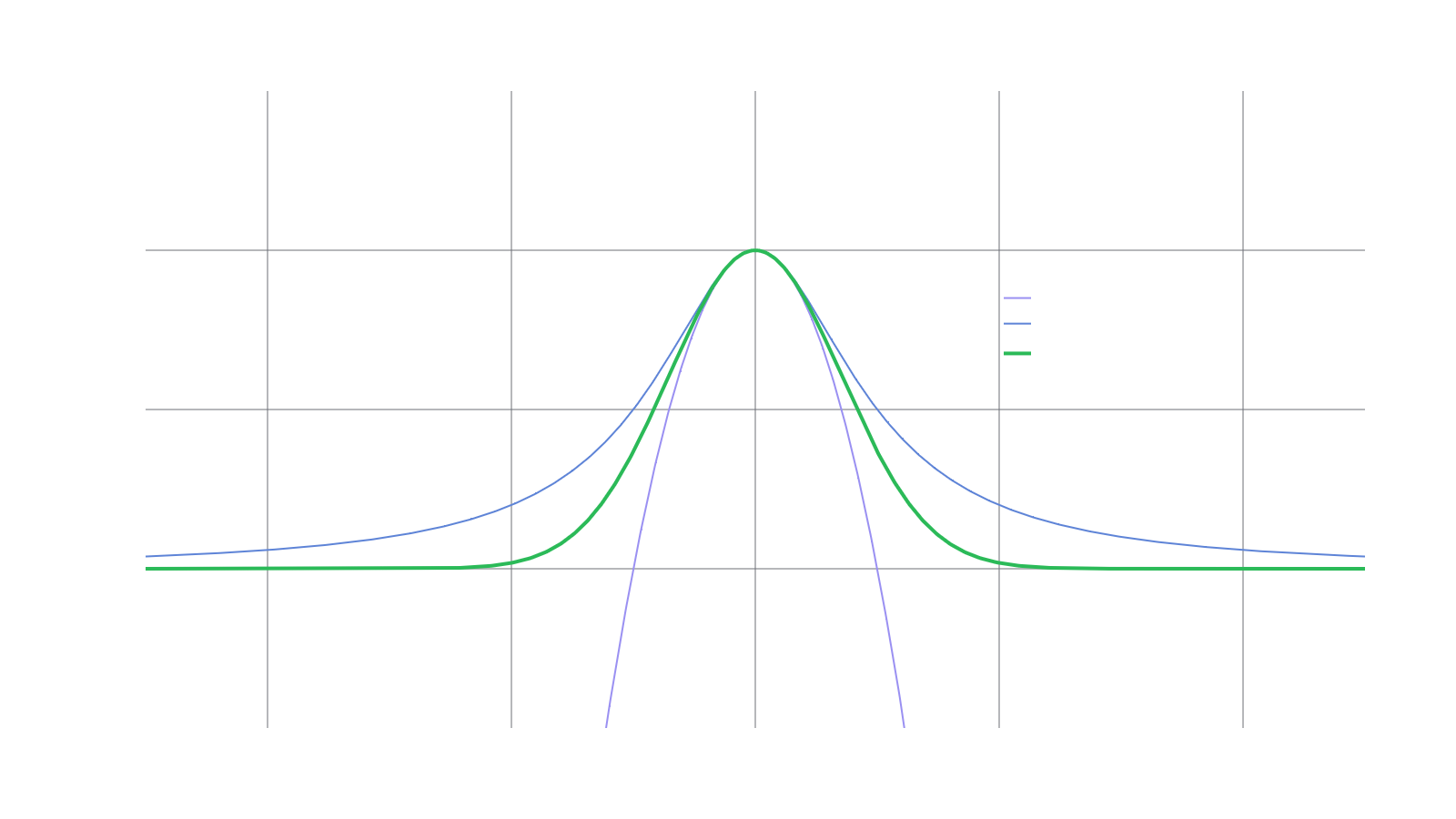
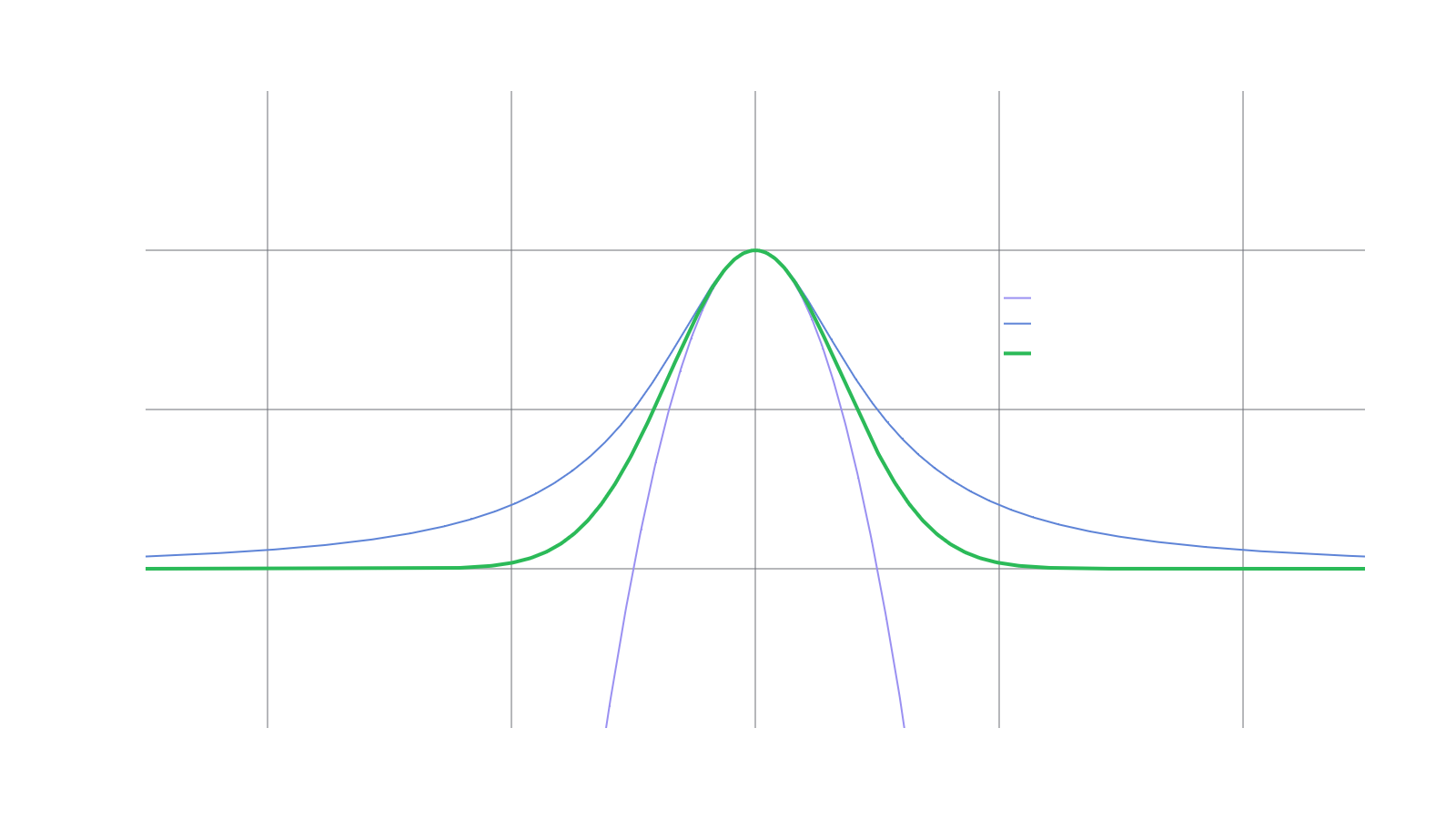
Aside from computational efficiency, another benefit of using rational functions is the ability to express degenerate function behavior such as singularities (poles/infinities), boundedness, or asymptotic behavior. Qualitatively, the functions and look very similar on all of and the approximation fares far better than outside of a narrow range. See the labeled curves in the following figure.
Continued fraction approximations
The degree of accuracy for a given approximation should be selected based on need and with respect to environmental constraints. The approximations in solstat are an economized continued fraction expansion:
This is typically a faster way to compute the value of a function. It's also a way of definining the Golden Ratio (the most irrational number):
Finding continued fraction approximations can be done analytically or from Taylor coefficients. There are some specific use cases for functions that have nice recurrence relations (e.g., factorials) since they work well algebraically with continued fractions. The implementation for solstat is based on these types of approximations due to some special relationships defined later.
Finding and Transforming Between Approximations
Thus far this article has not discussed getting these approximations aside from the case of the Taylor series. In each case, an approximation consists of a list of coefficients (e.g., Taylor coefficients ) and a map to some expression with finitely many primitive function calls (e.g., a polynomial ).
The cleanest analytical example is the Taylor series since the coefficients for well-behaved functions can be found by computing derivatives by hand. When this isn't possible, results can be computed numerically using finite difference methods, e.g., the first-order central difference, in order to extract these coefficients:
However, this can be impractical when the coefficients approach the machine precision level. Also, Laurent series coefficients are determined the same way.
Similarly, the coefficients of a rational function (or Pade) approximation can be determined using an iterative algorithm (i.e., akin to Newton's method). Choose the order and of the numerator and denominator polynomials to find the coefficients. From there, many software packages have built-in implementations to find these coefficients efficiently, or a solver can be implemented to do something like Wynn's epsilon algorithm or the minimax approximation algorithm.
All of the aforementioned approximations can be transformed into one another depending on the use case. Most of these transformations (e.g., turning a polynomial approximation into a continued fraction approximation) amount to solving a linear problem or determining coefficients through numerical differentiation. Try different solutions and see which is best for a given application. This can take some trial and error. Theoretically, these algorithms seek to determine the approximation with a minimized maximal error (i.e., minimax problems).
Breaking up the approximations
Functions also come along with domains of definition . Intuitively, the error for functions with bounded derivatives has an absolute error proportional to the domain size. When trying to approximate over all of , the smaller the set , the better. It only takes points to define a polynomial of degree . This means a domain with points can be perfectly computed with a polynomial.
For domains with infinitely many points, reducing the measure of the region approximated over is still beneficial especially when trying to minimize absolute error. For more complicated functions (especially those with large derivative(s)), breaking up the domain into different subdomains can be helpful.
For example, in the case of , a 5th degree polynomial approximation for has max absolute error . After splitting the domain into even-sized pieces, the result is and , which is used in the original algorithms to determine two distinct sets of coefficients for their approximations. In the domain of interest, and only have in error. Yet, if extended outside of , the error will have increased to . Each piece of the function is optimized purely for its reduced domain.
Breaking domains into smaller pieces allows for piecewise approximations that can be better than any non-piecewise implementation. At some point, piecewise approximations require so many conditional checks that it can be a headache, but this can also be incredibly efficient. Classic examples of piecewise approximations are piecewise linear approximations and (cubic) splines.
Ethereum Environment
In the Ethereum blockchain, every transaction that updates the world state costs gas based on how many computational steps are required to compute the state transition. This constraint puts pressure on smart contract developers to write efficient code. Onchain storage itself also has an associated cost!
Furthermore, most tokens on the blockchain occupy 256 bits of total storage for the account balance. Account balances can be thought of as uint256 values. Fixed point math is required for accurate pricing to occur on smart contract based exchanges. These libraries take the uint256 and recast it as a wad256 value which assumes there are 18 decimal places in the integer expansion of the uint256. As a result, the most accurate (or even "perfect") approximations onchain are always precise to 18 decimal places.
Consequently, it is of great importance to be considerate of the EVM when making approximations onchain. All of the techniques above can be used to make approximations accurate near in precision and economical simultaneously. To get full precision, the computation for rational approximations would need coefficients with higher than 256bit precision and the associated operations.
Solstat Implementation
A continued fraction aproximation of the Gaussian distribution is performed in Gaussian.sol. Solmate is used for fixed point operations alongside a custom library for units called Units.sol. The majority of the logic is located in Gaussian.sol.
First, a collection of constants used for the approximation is defined alongside custom errors. These constants were found using a special technique to obtain a continued fraction approximation that is for a related function called the gamma function (or more specifically, the incomplete gamma function). By changing specific inputs/parameters to the incomplete gamma function, the error function can be obtained. The error function is a shift and scaling away from being the Gaussian CDF .
Gaussian
The gaussian contract implements a number of functions important to the gaussian distributions. Importantly all of these implementations are for a mean and variance .
These implementations are based on the Numerical Recipes textbook and its C implementation. Numerical Recipes cites the original text by Abramowitz and Stegun, Handbook of Mathematical Functions, which can be read to understand these functions and the implications of their numerical approximations more thoroughly. This implementation is also differentially tested with the javascript Gaussian library, which implements the same algorithm.
Cumulative Distribution Function
The implementation of the CDF aproximation algorithm takes in a random variable as a single parameter. The function depends on helper functions known as the error function erf which has a special symmetry allowing for the approximation of the function on half the domain .
It is important to use symmetry when possible!
Furthermore, it has the other properties:
The reference implementation for the error function can be found on p221 of Numerical Recipes in section C 2e. This page is a helpful resource.
Probability Density Function
The library also supports an approximation of the Probability Density Function(PDF) which is mathematically interpeted as . This implementation has a maximum error bound of of and can be refrenced here. The Gaussian PDF is even and symmetric about the -axis.
Percent Point Function / Quantile Function
Aproximation algorithms for the Percent Point Function (PPF), sometimes known as the inverse CDF or the quantile function, are also implemented. The function is mathmatically defined as , has a maximum error of , and depends on the inverse error function ierf which is defined by
and has a domain in the interval along with some unique properties:
Invariant
Invariant.sol is a contract used to compute the invariant of the RMM-01 trading function such that is computed in:
This can be interpretted graphically with the following image:
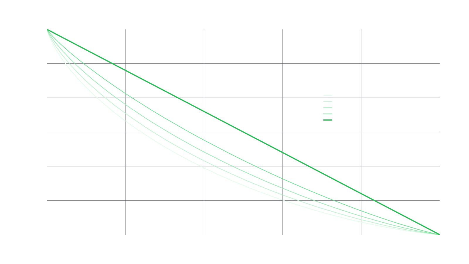
Notice the need to compute the normal CDF of a quantity. For a more detailed perspective on the trading function, take a look at the RMM-01 whitepaper.
Solstat Versions
Solstat is one of Primitive's first contributions to improving the libraries availible in the Ethereum ecosystem. Future improvements and continued maintenance are planned as new techniques emerge.
Differential Testing
Differential testing by Foundry was critical for the development of Solstat. A popular technique, differential testing seeds inputs to different implementations of the same application and detects differences in the execution. Differential testing is an excellent complement to traditional software testing as it is well suited to detect semantic errors. This library used differential testing against the javascript Gaussian library to detect anomalies and varying bugs. Because of differential testing we can be confident in the performance and implementation of the library.